Adjust Valuation Multiple for Growth

If one equity is valued at 15x P/E, and another at 10x P/E, is the latter a bargain?  To answer this question we should adjust for growth.

Adjusting a valuation multiple (such as P/E or EV/EBITDA) is frequently done by dividing by growth — such as with the common P/E/G multiple.

We can do better…

Don’t Divide by Growth

Nearly universally we measure the value of growth using some version of the Gordon growth model.   We notice that value doesn’t change linearly with growth, so adjusting a valuation multiple to  control for growth by dividing by growth (as is done with P/E/G) leads to bias.  Damodaran details this effect.

Apart from the issue with linearity, another important problem with the PEG approach is that it assumes the stated growth lasts forever.  However,

• Empirical research indicates that a firm’s outperformance (relative to its peer group) lasts at most 5 years, and usually less
• Microeconomic and financial theories suggest that a firm’s long-run growth can never be above that of the surrounding economy.  (In the US, long-run nominal growth averages 5.5%.)

 

Recipe

So we desire a more principled technique to adjust valuation multiples for differing growth assumptions.  To do so we will convert the growth projections of the company (which start high, and then revert to 5.5%) into a value-equivalent stream of flows which grow at a steady rate.  We then re-value this adjusted stream of flows using a common growth assumption (again, 5.5%) to see what the firm’s multiple would be if it were only growing at this common rate.

1. Determine a model for valuing long-run growth, which implies a stream of flows (which grow at different rates over time)
2. Determine a stream of flows (whether these flows be dividends, FCF, or whatever you choose) which, under constant growth, produce a value equivalent to that implied by the current multiple
3. Re-value this stream of flows under a common growth assumption

Variations of the Gordon growth model that allow for changing growth include 2-stage, 3-stage, and H-model (all described by Damodaran.)

We use the H-model, which assumes that the initial growth rate reverts linearly to the sustainable growth rate.  The H-model also provides a closed-form valuation equation.

To simplify the algebra, revise the above recipe as follows:

1. Input sustainable growth rate “g”, initial-period growth rate “g_init”, number of periods after which initial growth reverts to sustainable growth rate “t”, and unadjusted multiple “M”
2. From the H model, impute the (1/(r-g)) annual discount rate:  M / (1 + g + H(g_init – g))
3. This in turn gives us r, the riskiness of our firm.
4. Now value a new firm, with the same risk (r) as the subject firm, but which grows steadily at g.  We can use the simple 1-period Gordon model:  (1+g)/(r-g)

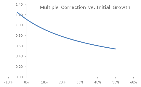
Assuming 4-year growth reversion period, sustainable growth at 5.5%, we can create the following chart (which shows initial growth rate on X axis, and multiple correction factor on the Y axis):

Loose Ends

1. Equity analysts, on average, predict growth at ~11%.  Since growth averages 5% or so, you should haircut analyst growth estimates by 50%.  (However, if investor expectations, and thus multiples, take these growth estimates at face value, you should use them in the above procedure without modification.)
2. We implicitly assumed that the firm’s risk doesn’t change.  If growth is expected to begin high and then fall, we should expect risk to decline as well.